Lambda Calculus: A Preliminary View
“You are the only problem you will ever have and you are the only solution.”
— Bob Proctor
Prologue
I’ve been struggling making up the missing background knowledge for my research, which is not something very enjoyable. I always hate formulas and mathematical proofs. However, I did find something interesting among those boring stuffs, which is the theory behind functional programming.
This is a reflection when I was learning MIT 6.820 Fundamentals of Programming Analysis. This post roughly covers lecture 1 to 3.
Basics on Functional Programming
First of all, there is some basic concepts in functional programming.
Free/Bound Variables
In functional programming, the function is, the function we know. There is nothing special. A function consists of name, arguments and a body, where there are variables (or identifiers) as the arguments or in the body. Variables are the actual operands, so we need to define them more carefully.
There are two kinds of variables, one is free, the other is bound. It is easy to tell them apart, where bound variables are those appear in the arguments of a function, and the others are free variables. Bound variables are those you must provide to invoke (or apply) a function, while free variables are captures from the context. For example, in the following func function below, x and y are bound variables, and a and b are free variables.
1 | func x y = x * a + y * b |
Bound variable is also known as formal parameter.
Renaming
As an experienced programmer, you may not notice the existence of renaming although you know it. Given the C snippet below, you immediately know that the inner a and the outer a are different, even though they have the same lexeme.
1 | function () => { |
TypeScript has concepts like closure and types, which makes it a good substitution for pure functional programming languages like Haskell if you don’t have prior knowledge of the latter.
Although discouraged, in real programming, we can have two identifiers using the same name and let one hides another. However, in theory, to avoid confusion (at least I think so), renaming them is a better idea. So, we have $\alpha$-renaming. After $\alpha$-renaming, the above code snippet will become as below.
1 | function () => { |
Do pay attention to it, as this renaming process will be used later for substitution.
As renaming is to avoid name confliction, one can only rename bound variables, and should not introduce new name confliction.
Type System
No matter it is static type or dynamic type, there is always type. In functional programming, Hindley—Milner type system is often used.
Informally, the type of an expression is either OUT or IN -> ... -> IN -> OUT. If it is a variable, then apparently, it has a fixed type. For a function, it’s type is defined by what it takes in and what it gives out. Given an example below, it should be easy to understand.
1 | add : Number -> Number -> Number |
It is fun to think that, give a function, you can either provide all arguments at once, or provide arguments one by one. And both can have the final answer.
This type system is natural for pure functional programming languages. But if you only do functional style programming in other languages, you may need to use the so-called curried function to achieve this. For example, in TypeScript, you can do this. The idea is construct new functions and capture existing arguments as free variables.
1 | function add(a: number, b: number): number { |
This trick is useful to partial initialize template variables in TypeScript.
The $\lambda$ Calculus
To bring our topic to a higher level, we have $\lambda$ calculus. It is the abstract form of functional programming.
Syntax
The syntax of pure $\lambda$ calculus is given below, which uses a common grammar notation. It may seem a bit weird at first to see something like $\lambda x.E$, but you can take it a equivalent of function (x) => E. As for the application, the left E should reduce to an abstraction (a.k.a. function), so the right part can be the argument.
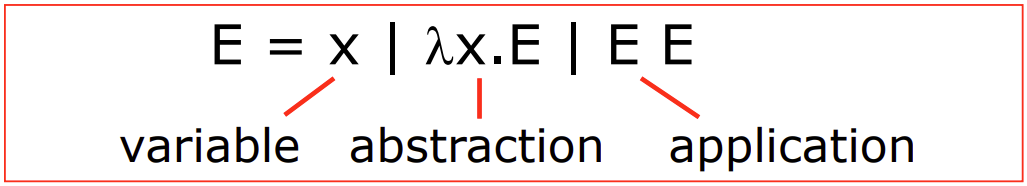
This grammar definition is simple and contains left recursion, so you may already notice that it is ambiguous. Therefore, we have an extra rule that the scope of the dot in an abstraction extends as far to the right as possible. Now, it is not ambiguous.

Combinator
The definition for free and bound variables also applies here. In $\lambda x.E$, $x$ is a bound variable, and all other variables in $E$ are free variables.
However, we have a new concept here. If a $\lambda$ calculus (or $\lambda$ expression) comes without free variable, it is then called a combinator or a closed $\lambda$ expression.
Substitution
One reason I don’t like theory is that, in theory, people just name the same thing with different words, and make simple things complex.
Here, substitution is simply renaming of variables, and we note it with $[y/x]$, meaning replacing all $x$ to $y$. So, $E[y/x]$ is replacing all $x$ to $y$ in $E$. Then what is it used for? Well… it is the abstraction of function application. For example, as given below, we pass $E_a$ as the argument to an abstraction.
$$
(\lambda x.E) E_a \rightarrow E[E_a/x]
$$
A bit too abstract? Take a TypeScript example below.
1 | (function (x) => x + 1)(a) // before: E = x + 1, Ea = a |
After application, arguments becomes substitution, which follows \beta-substitution. The substitution matches exact variable name, so it is possible that nothing changes after substitution. In short, the rule of \beta-substitution is given below. Notice that, x and y here are expressions, which means they can be variables or functions.
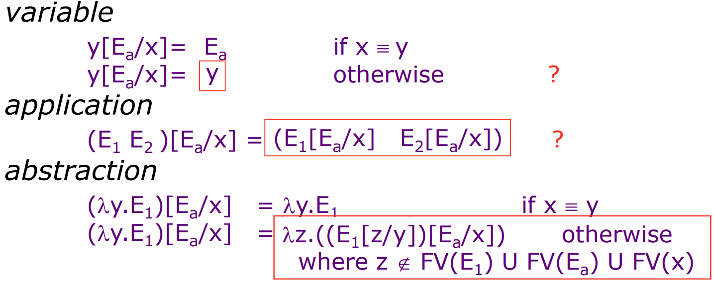
Don’t worry, the question marks in the image above do not mean they are wrong.
As for the application, it is like, you calls the function with $x$, then all inner functions/expressions will use this $x$ if they use $x$ as a variable (either free or bound).
As for abstraction, it makes sense that if you substitute a bound variable, it makes no difference as it is just an argument. However, in other case, you should be careful not to introduce name confliction. That is to say, if $E_a$ contains $y$, it will “contaminate” $\lambda y.E_1$, so we first need to ensure the bound variable $y$ in $E_1$ does not appear as a free variable in $E_a$.
Why only ensure $z$ is not a free variable? Because bound variables have scopes, so it is OK to have nested bound variables, although not friendly for reading.
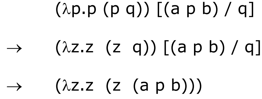
Here is an example using $\beta$-substitution, from which you can see something bad will happen if we do not rename $p$ in the first place.
Reduction
The $\lambda$ calculus it self can be a reduction system, in which we reduce the expression by applying functions. Some terms to keep in mind. $\alpha$-rule is essentially the renaming rule, like what you do to rename a parameter. $\beta$-rule is covered just now. Take greater attention to redex (reducible expression) and normal form here as we will talk about it real soon.
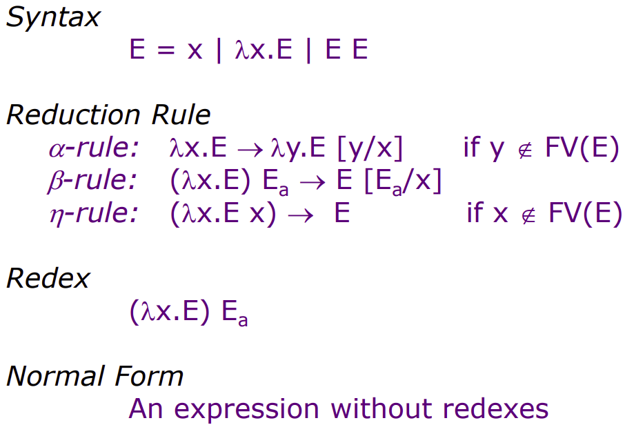
We will not talk about $\eta$-rule.
Here is an example on reduction. Now you can see function as argument, which is normal in functional programming.
A possible reduction is given below. Because we have confluence, the order of reduction does not matter.
$$
\begin{align}
\begin{split}
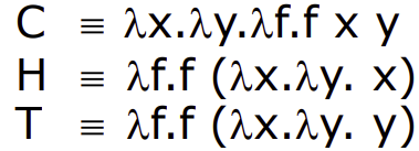
& H (C \space a \space b) \newline
\rightarrow \space & (\lambda f.f(\lambda x.\lambda y.x))(C \space a \space b) \newline
\rightarrow \space & (C \space a \space b) (\lambda x.\lambda y.x) \newline
\rightarrow \space & ((\lambda x.\lambda y.\lambda f.f \space x \space y) \space a \space b)(\lambda x.\lambda y.x) \newline
\rightarrow \space & (\lambda f.f \space a \space b)(\lambda x.\lambda y.x) \newline
\rightarrow \space & ((\lambda x.\lambda y.x) \space a \space b) \newline
\rightarrow \space & a
\end{split}
\end{align}
$$
Confluence
Just mention it briefly. Confluence means that if there is $E \rightarrow E1$ and $E \rightarrow E2$, then there is $E1 \rightarrow E3$ and $E2 \rightarrow E3$, so that eventually we still have $E \rightarrow E3$. It is also called Church-Rosser Property of a reduction system. $\lambda$ calculus has such property, but not all reduction systems.
Reduction Strategy
Like what we learnt in Compiler Technology course, we have left-most (normal) reduction and right-most reduction. Under the setting of $\lambda$ expression, they are also called normal order and applicative order.
It is interesting, as for compilers, we use normal reduction to parse the abstract syntax tree. However, in most programming languages (e.g. C, TypeScript), we use applicative order to evaluate an expression (i.e. prepare all arguments before calling a function).
Term
Don’t forget why we are learning all these. We are part of our journey to program analysis, and one goal is to understand the meaning of a program. And to do this, we need to first define the meaning of an expression, or term.
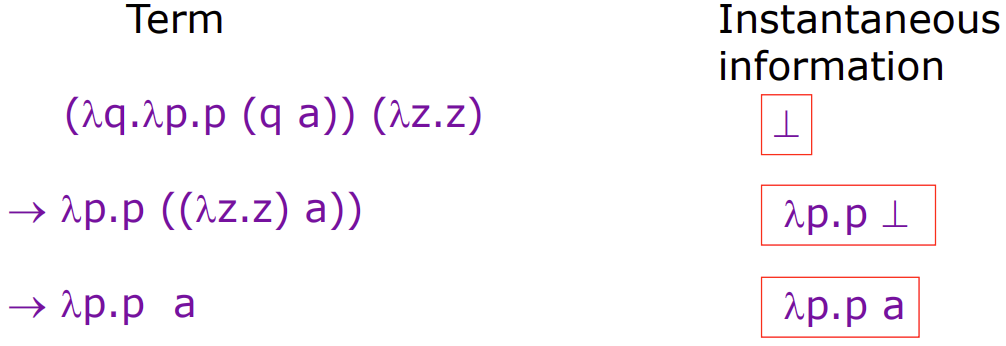
A redex will be reduced because it is not the final form, so we define it to carry no information ($\bot$). Then, the meaning of a term is obtained by replacing all redex in it with $\bot$, which is called instantaneous information. See below, the information monotonically increases by $\beta$ reduction.
So, it seems the meaning of a term is defined by its normal form. However, not all terms has normal form, for example, the term $\Omega$ can’t be reduced to a normal form, and each reduction result is still itself. Also, since the syntax of $\lambda$ calculus is not ambiguous, one term won’t have multiple normal forms.
$$
\Omega = (\lambda x.x \space x) (\lambda x.x \space x)
$$
This is a very special term, which is also very useful. We’ll see it again later.
Normal Form
The reduction will lead an expression to its normal form (unless it is like $\Omega$). Since we are talking about normal form, we imply the usage of normal reduction. Based on normal form, there are two other variations that interests us.
Head normal form (HNF): A term in which the head is not a redex. It represents the information content of an expression.
$$
\begin{split}
x & \in HNF \newline
x \space E_1 \space E_2 … E_n & \in HNF \newline
\lambda x.E & \in HNF \space (if \space E \in HNF) \newline
\end{split}
$$
Weak head normal form (WHNF): A term in which the left most application is not a redex. This is useful in practice. Suppose that you have an expression, if it is a variable or function, you know what it is. But if it is a function call, you cannot determine what it is unless you really call it and get its result, and the result is either a variable or function.
$$
\begin{split}
x &\in WHNF \newline
x \space E_1 \space E_2 … E_n &\in WHNF \newline
\lambda x.E &\in WHNF
\end{split}
$$
The Y Combinator
There is a wonderful blog you can refer to: The Y Combinator.
In mathematics, there is concept of fixed point, which is $x = f(x)$. This can be an interesting property in $\lambda$ calculus when there is recursion. Normally, when we have recursion, we will write something like this: fact(n) => n * fact(n - 1), which is
$$
fact = \lambda n.n*fact(n-1)
$$
In $\lambda$ calculus, we can abstract it to be
$$
\lambda f.\lambda n.n * f(n - 1) = \lambda f.(\lambda n.n * f(n - 1))
$$
Now, it becomes a function that takes a function (f), and returns another function which takes the original argument (n) and invokes the argument function (f).
It sounds really messy, so what are we doing here? Take a breath, and you may notice that the recursion is gone. Instead, we are calling “another” function. But being a recursion problem in nature, this “another” function should behave the same. So, how is this done?
Fixed Point
You apply a function, and get it back. In this case, you are playing with fixed point. Just now, we met a special $\lambda$ expression which always reduce to it self:
$$
\Omega = (\lambda x.x \space x) (\lambda x.x \space x)
$$
Then, if we make a little modification, it becomes
$$
\begin{align}
\begin{split}
\Omega_F & = (\lambda x.F(x \space x)) (\lambda x.F(x \space x)) \newline
& = F \space ((\lambda x.F(x \space x))(\lambda x.F(x \space x))) \newline
& = F \space \Omega_F \newline
& = F \space (F \space \Omega_F)
\end{split}
\end{align}
$$
We can see that $\Omega$ is a fix point of $F$. Now, we abstract it and get the Y Combinator
$$
Y = \lambda f.\Omega_F[f/F] = \lambda f.(\lambda x.f(x \space x)) (\lambda x.f(x \space x))
$$
Then given any function $F$, we have $YF = \Omega_F$ being the fixed point of $F$, i.e. $YF = F(YF)$. Suppose our $F$ returns $\lambda n.E$, we have
$$
\begin{align}
\begin{split}
Y \space F \space n &= (YF) \space n \newline
&= ((\lambda x.F(x \space x)) (\lambda x.F(x \space x))) \space n \newline
&= F \space ((\lambda x.F(x \space x)) \space (\lambda x.F(x \space x))) \space n \newline
&= F \space (Y \space F) \space n
\end{split}
\end{align}
$$
Depending on the behavior of $F$, it can call $YF$ so that the invocation goes on and on, until $F$ stops calling $YF$ with certain value of $n$.
Type?
Be careful when you reason the types here. Although we are having the same identifier $F$, each instance has different type. Assuming that $F$ has type $T \rightarrow R$. Then, we have the following types. The type given is the head identifier’s type.
$$
\begin{align}
\begin{split}
F_0 :& \space T \rightarrow R \newline
YF_0 :& \space (T \rightarrow R) \rightarrow R \newline
F_1(YF_0) :& \space ((T \rightarrow R) \rightarrow R) \rightarrow R \newline
F_2(F_1(YF_0)) :& \space (((T \rightarrow R) \rightarrow R) \rightarrow R) \rightarrow R
\end{split}
\end{align}
$$
So, we can see that even though they are all $F$, their types are different. The only type that is the same is the return type. Thus it is a problem for static typed languages.
About Y Combinator
The $x \space x$ in the Y Combinator might be confusing. It is a self application, and does not mean that $F$ takes two arguments. Instead, it means $F$ takes one argument which is the result of the expression $x \space x$. And as indicated, the result of $x \space x$ is $Y \space F$, the fixed point. Hence, $F$ eventually takes $F’$, and returns $\lambda n.E$, where $F’ \in E$ (it would be funny if $F’ \notin E$), so that the chain goes on.
You may wonder, how does this chain stop? In common programming languages, the runtime uses applicative order (check Reduction if you forget it), which means all arguments will be resolved before calling a function. In this case, We will end up resolving $YF$ forever and never have the chance to go into $F$. In other words, these languages only accept normal form.
However, many functional programming languages use normal order reduction even for arguments. In these languages, weak head normal form is accepted. Therefore, the runtime won’t evaluate $YF$ further until necessary, which is also called lazy evaluation. So that $F$ can take $YF$ (WHNF) as it is, return $\lambda n.E$, and only evaluate $YF$ in the invocation of $\lambda n.E$ if needed.
You will get a clearer view of it in the following implementation.
Implementation of Y Combinator
The concept is always abstract, so let’s make it concrete. Ultimately, what we want is $YF = F(YF)$, so we just need to ensure this property.
First, for clarity, we define an alias for function that takes one argument.
1 | type Func<T, R> = (arg: T) => R; |
Take factorial calculation as the example. The recursive version (recursive factorial) would be as follows, which is $\lambda x.E$. Here, rfact is a free variable as it is captured outside.
1 | const rfact = (n: number): number => n == 0 ? 1 : n * rfact(n - 1); |
However, we don’t want direct recursion, i.e. we don’t want to capture rfact in itself. Now, if we abstract rfact, then rfact becomes a bound variable f. Essentially, our rfact is now a formal argument of fact, and fact returns rfact. The direct recursion is eliminated.
1 | const fact = (f: Func<number, number>): Func<number, number> => (n => n == 0 ? 1 : n * f(n - 1)); |
From certain point of view, our fact is now a generator.
Then, let’s think about the Y Combinator. From the implementation’s view, it is quite straight forward. We just need to make sure $YF = FYF$. So, it can be rather simple.
1 | const Y = (f: any): any => f(Y(f)); |
And this is it, now we can calculate factorial using Y(fact).
1 | console.log(`factorial(${5}) = ${Y(fact)(5)}`); |
This is it? No direct recursion?
Looking back, Y in fact recursively provides the f in fact. When ever fact calls f, it is calling Y(fact), which yields another Y(fact), thus achieving recursion without direct recursion in fact.
Lazy Evaluation
However, when you actually run the code, you will immediately see stack overflow. This is what I mentioned earlier. TypeScript uses applicative order for argument evaluation, so Y will result in infinite recursion on application.
Luckily, for languages using applicative order evaluation, there is a workaround if they support lambda expression. We want to prevent the immediate invocation of Y in f(Y(f)). To do so, we can delay it into a lambda function call.
1 | const Y = (f: any): any => f((x: any) => Y(f)(x)); |
Now, Y won’t be invoked unless the lambda expression is invoked. Problem solved. By the way, you can add type hint for Y.
1 | const Y = <T, R>(f: Func<Func<T, R>, Func<T, R>>): Func<T, R> => f((x: T) => Y(f)(x)); |
No Recursion?
Remember what we want at the very beginning? To eliminate direct recursion. However, even we did it for fact, there is still direct recursion in Y. So our job is not finished yet. Let’s look at the equation again. Just now, we used $(4)$, so there is Y inside Y. Hmm, so the solution is quite clear — we can use $(2)$ or $(3)$.
$$
\begin{align}
\begin{split}
Y \space F \space n &= (YF) \space n & (1) \newline
&= ((\lambda x.F(x \space x)) (\lambda x.F(x \space x))) \space n & (2) \newline
&= F \space ((\lambda x.F(x \space x)) \space (\lambda x.F(x \space x))) \space n & (3) \newline
&= F \space (Y \space F) \space n & (4)
\end{split}
\end{align}
$$
Since $(3)$ is derived from $(2)$, we just use the simpler one. Follow the equation, we get this. And we are done, again.
1 | const Y = (f: any): any => ((x: any): any => f(x(x)) ((x: any): any => f(x(x)) |
It may take you quite a while to get the idea.
Now you may wonder, can we add type annotations to it like we did before? The answer is yes, but no. The recursion cannot be totally eliminated, which now goes to the type. If you want to add types, this is what you will get. The last any in recursive and is unable to be expressed in TypeScript other than using any.
1 | const Y = <T, R, U = Func<T, R>>(f: Func<Func<T, R>, U>): U => |
To my limited knowledge of TypeScript, we can’t have recursive definition of template arguments. But if it is possible, do leave a comment below.
That should be all about the Y Combinator I have to talk about.
Epilogue
Isn’t it fun? No? Well, I guess you are right. But it indeed provides a different angle towards programming. And it is a new experience from theory to implementation. And, it takes a lot of time. ᓚᘏᗢ